Unraveling Deep & Cross Networks

Explaining an effective recent method for automatic feature crosses

My colleague, Tim Huang, wrote an excellent blog about his recent work at Thumbtack applying Deep & Cross Networks (DCNs): Leaves to Neurons: Using Deep-Cross Networks for Ranking Search Results. It’s a good read; go check it out! This is a fitting time for me to share some of my notes on DCNs. When I try to learn something that doesn’t come to me intuitively, I like to simplify it into its most basic version and break it down into smaller pieces.

The problem we want to solve is how to automatically find multiplicative interactions (“crosses”) in an ML model. To use a painfully reductive and geometric example, let’s say we wanted to predict how much paint we need in order to paint a wall, and we have length and height as features. Length and height do not matter on their own, but their product sure does. As humans we have domain knowledge and could easy construct an area feature that equals length times height, but in other domains we won’t always know the correct relationships between features and labels. We want our algorithms to discover these relationships on their own.

This topic has a long history in neural networks, but we’re going to start in recent years. The Deep & Cross Network (DCN) is a method shared by Wang et al. (2017) from Google [1]. Later on, Google substantially changed the method in Wang et al. (2020) and released DCN-V2 [2]. In 2021 Weibo released a conceptually similar architecture, MaskNet, in Wang et al. (2021) [3].¹ I’ll specifically talk about DCN-V2 here, breaking it down into simple parts. For a look at how these fit within a broader history of feature interaction methods, see this succinct write-up by Sidney Fletcher, in the context of Twitter adopting MaskNet.

With Google, Weibo, Twitter, and others using these types of models, they're worth looking into.

First step in unraveling: what is a deep cross network? Simply enough, it’s any neural network that has cross layers.²

How a cross layer works

So let’s talk about what a cross layer is. 

Figure 2 from Wang et al. (2020).

This diagram shows a three-valued input, but the concept extends to other sizes. This could match the example from TensorFlow documentation, where X represents (country, banana, cookbooks). In this diagram, X₀ is the vector of inputs (e.g. the values for country, banana, and cookbooks), X_i is the value at layer i, and W and b are weights that we learn. So we have three inputs (in this example), we have three outputs, and we use 12 parameters (3² + 3) to learn.

Consider layer 1, the first cross layer. For that matter, it could easily be the only cross layer.

Explicitly describing the first cross layer, modified from Figure 2 of Wang et al. (2020)

Let’s set bias to 0 for now, setting it aside for later:

T first layer without a bias term, modified from Figure 2 of Wang et al. (2020)

The circle with a dot in it is element-wise multiplication (the Hadamard product), in contrast to the x which is matrix multiplication.

I’m going to unravel DCNs literally, by expanding the linear algebra into component equations. I’ll describe the X’s individually with a second subscript, as X_0,1, X_0,2, and X_0,3, counting from 1, and I’ll use two subscripts for W to indicate the two dimensions.³ If these equations or others wrap and are hard to read, consider opening the post (and not just the email) on a computer instead of a phone.

X1,1 = X0,1 * (W1,1 * X0,1 + W1,2 * X0,2 + W1,3 * X0,3) + X0,1
X1,2 = X0,2 * (W2,1 * X0,1 + W2,2 * X0,2 + W2,3 * X0,3) + X0,2
X1,3 = X0,3 * (W3,1 * X0,1 + W3,2 * X0,2 + W3,3 * X0,3) + X0,3

Putting the X₀ into the parentheses and adding some spaces for alignment:

X1,1 = (W1,1 * X0,12      + W1,2 * X0,1 * X0,2  + W1,3 * X0,1 * X0,3) + X0,1
X1,2 = (W2,1 * X0,2 * X0,1 + W2,2 * X0,22       + W2,3 * X0,2 * X0,3) + X0,2
X1,3 = (W3,1 * X0,3 * X0,1 + W3,2 * X0,3 * X0,2  + W3,3 * X0,32)      + X0,3

Every element of X is crossed with every other element of X, with a weight on it. They’re actually crossed twice each. And they’re also crossed with themselves, giving us squared features.

Why does DCN-V2 use so many parameters?

The square W matrix seems a bit wasteful. It has 9 weights to learn (in our 3-input example). 3 of them are squared features, which seems unnecessary in a neural network. The squared features are even less necessary in the use case of the paper, where most features are binary. The other 6 are 2 parameters for each of 3 crosses. Why not just use 3 parameters, instead of 9? In the general case, instead of k², we could use k * (k - 1) / 2 crosses, which is approximately half the parameters as we reach large k.

I suspect part of the answer is that the square matrix is easy to implement and works well on our frameworks with efficient matrix multiplication.

We also get a little more expressiveness out of the cross layers. Remember that there is a b vector added in. Since b can vary, we’re not exactly replicating the crosses twice. We’re able to shift them. Although it’s a bit of an odd shift, because it’s not a cross-specific one but rather it shifts a group of crosses. 

We also merge the crosses within each layer, in the example above still ending up with 3 output features rather than 9. So even though we use X_0,2 * X_0,1 twice, for example, in each use it is combined with a different set of other crosses.

Maybe feature crosses as a layer are better than pre-computing cross features for memory consumption reasons. k * (k - 1) / 2 features is a lot, potentially consuming significant memory if we have to do it for each of n rows. We still need to store k² + k weights per cross layer, but at least that’s not n * k * (k - 1) / 2 stored features.

Why do we add X_i back in?

This is a very ResNet-inspired idea. The authors think of the cross layer as fitting the residual. If W and b are 0, then X_i+1 = X_i and the layer is a no-op (non-operation, or the identity function). That’s somewhat the default case. Neural networks are usually initialized with small random weights, and those might net out to approximately a 0 effect. In DCN-V2 they did that for the multiplicative weights, and explicitly initialized all the bias terms to 0. So the model doesn’t really have to modify those weights much to learn a no-op if a no-op is what’s needed. That could be the case in models (or parts of models) where feature crosses aren’t really useful.

The other thing this does is that as we propagate each layer into the next cross layer, stacking cross layers, the model can (for example) ignore cubic and other higher-order features (give them 0 coefficients) if it so chooses.

The output is the same dimensionality as the input

Related to the above, there’s no reason why the cross layer had to necessarily output the same number of elements as the input. But it’s a nice property, such that if we have small weights we can learn the identity function. We’re not shrinking or expanding the dimensionality between layers. We can stack as many as we want, increasing complexity but keeping dimensionality the same. This concept is also popular in modern transformer-based models, where transformers maintain dimensionality and can be stacked to any chosen depth.

…which helps us avoid parameters later on

Another disadvantage of creating explicit cross features is that in fully connected (“dense”) networks we would create as many subsequent parameters for each resulting cross as we have neurons in the next layer. E.g. if the next layer has w neurons then with k * (k - 1) / 2 crosses we’d end up with w * k * (k - 1) / 2 additional weights to learn. By isolating the crossing into its own part of the network, we can avoid creating too many parameters. We could do it anyways by specifying a less-than-fully connected layer, but that would require more manual setup.

How do deeper layers work?

Again setting aside b for now. 

X1,1 = X0,1 * (W1,1 * X0,1 + W1,2 * X0,2 + W1,3 * X0,3) + X0,1
X1,2 = X0,2 * (W2,1 * X0,1 + W2,2 * X0,2 + W2,3 * X0,3) + X0,2
X1,3 = X0,3 * (W3,1 * X0,1 + W3,2 * X0,2 + W3,3 * X0,3) + X0,3

Let’s use V for the second layer’s weights, and .* to indicate the element-wise product:

X2 = X0 .* (V * X1) + X1

I’ll only expand one of the three rows:⁴

X2,1 = X0,1 * (V1,1 * X1,1 + V1,2 * X1,2 + V1,3 * X1,3) + X1,1

Expanded to:

X2,1 = X0,1 * (V1,1 * (X0,1 * (W1,1 * X0,1 + W1,2 * X0,2 + W1,3 * X0,3) + X0,1) + V1,2 * (X0,2 * (W2,1 * X0,1 + W2,2 * X0,2 + W2,3 * X0,3) + X0,2) + V1,3 *(X0,3 * (W3,1 * X0,1 + W3,2 * X0,2 + W3,3 * X0,3) + X0,3)) + X1,1

Expanded more and replacing X_1,1 with its components:

X2,1 = 
X0,1 * V1,1 * (X0,1 * (W1,1 * X0,1 + W1,2 * X0,2 + W1,3 * X0,3) + X0,1) + 
X0,1 * V1,2 * (X0,2 * (W2,1 * X0,1 + W2,2 * X0,2 + W2,3 * X0,3) + X0,2) +
X0,1 * V1,3 * (X0,3 * (W3,1 * X0,1 + W3,2 * X0,2 + W3,3 * X0,3) + X0,3) + 
X0,1 * (W1,1 * X0,1 + W1,2 * X0,2 + W1,3 * X0,3) + 
X0,1

So we can see that we keep the initial value of the feature (X_0,1), we keep the first order of interactions (X_0,1 * (W_1,1 * X_0,1 + W_1,2 * X_0,2 + W_1,3 * X_0,3)), and now we add in a second order of interactions that will now include cubed features and other three-part interactions.

Parameter reduction with U and V

In the DCN-V2 paper they modify the formula slightly, using U and V instead of W.

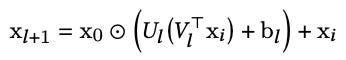
Equation 2 from Wang et al. (2020). I’m not sure why they use both i and l in the formula, since I believe they are the same.

If there are k features, W is a k x k matrix, while U and V have dimensions of k x r, for some r < k. X is a vector of k items, so when we transpose V and multiply by X_i we get a r x 1 matrix. When we multiply U by that result, we get a k x 1 matrix that we need for the subsequent addition with b and element-wise multiplication with X₀.

Why do we split the multiplication on X_i into two multiplications instead of just one? Because it reduces parameters. Consider the Criteo dataset (used in the paper) with 39 features. These 39 features expand to 1,027 because of embedding the categorical ones: 13 continuous features + 26 categorical features of 39 embedded dimensions each = 1,027 total inputs. W would have 1,027 * 1,027 = 1,054,729 parameters to learn. If instead we use U and V with r = 128, for example, then we have 1,027 * 128 + 1,027 * 128 = 262,912 parameters to learn, split across two matrices. That cuts the number of parameters down by 3/4.

This doesn’t come without cost: by reducing parameters and forcing reconstruction through matrix multiplication, we can’t (in the general case) perfectly recover the full W matrix. We can look at this as a compression mechanism, with all of the trade-offs of lossy compression. This is a widely applied technique, known as matrix factorization or matrix decomposition.

It’s good that they do this matrix factorization as part of model training itself, instead of learning a W and then later on trying to compress it. The optimal weights in U and V might change to reflect the reduced representative power. Figure 4b shows performance improving for any r (“We loosely consider the smaller dimension 𝑟 to be the rank”), implying that this compression does come with some cost:

Figure 4b from Wang et al. (2020), showing the cost of compression.

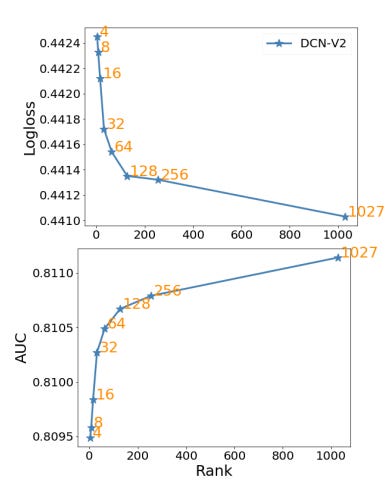
Log loss only decays from 0.4410 to 0.4416 when reducing from 1,027 features to a 64 dimension length, which might be a good trade-off for model fitting and inference speed. Although I’ll note that the alternatives they compare against have log loss in the range of 0.4420 to 0.4427, so a bit of compression compared to their best results does give up a lot of their reported performance gains.

DCN-V2 versus DCN V1

DCN only uses 2k parameters per cross layer, while DCN-V2 uses k² + k. DCN had a crafty way to include feature crosses without too many parameters. In this sense, DCN is craftier than DCNV2. Yet in DCN-V2 the authors move on from that and find that it’s worth it to have the much larger parameter space.

That’s definitely been a trend in ML for a long time now, of bigger and bigger models performing better. Looking at comparable model choices, I wonder if a natural extension is to expand the output dimensionality in the cross layer, instead of having it match the input layer. While it is very convenient that we can stack these and the output dimensionality never changes, maybe more expressiveness is just better.

The tutorial comparison is a little unfair

This is a bit of an aside, but the toy example in the first half of the TensorFlow DCN page shows much better performance for a DCN than a DNN. But the dataset is constructed to only have first order effects and cross effects. It’s really tailored to look good for DCNs.

I ran a linear regression with first order effects and the specific cross effects, and it crushed the DCN. It found the exact coefficients and gave almost 0 error—perhaps only floating point rounding. Awesome, right? Yet that’s not proof that we should always use linear regression. This example shouldn’t really convince us of anything. If we create data with a particular function and then use a restrictive model that can express those relationships, we should be unsurprised that the model does very well.

This demo is still a good example on how dense neural networks can struggle to fit certain functional forms like feature crosses. They can approximate crosses with enough width and depth, but it takes a lot of parameters and there is no guarantee that the relationship will be learned that well. 

But if anything, this example makes me curious: Why doesn’t the DCN do better than it does? Doesn’t it have enough expressive power to exactly fit this model? If anything this example could reduce my confidence in DCNs.

The second example (MovieLens) is more convincing, as is the other one from the paper (Criteo). The DCNs perform well. DCN V1 shows only marginal improvement—if you look past the very positive framing written in the paper—but DCN-V2 showed at least noticeable improvement on those datasets.

One lesson of all this: Functional forms still matter

A big lesson here is that feature engineering can still be valuable. The modern approach to feature engineering is layer engineering. What other types of relationships are poorly represented in typical DNNs? How about ratio features—should we invent ratio layers? Maybe we should have a library of smart layer types, including cross layers, and throw all of them into our models. Maybe we’re not very sufficiently diversified when we exclusively use dense layers.

Cross layers are a simple and effective way to incorporate multiplicative interactions into a neural network. They’re a good tool, and I expect they’ll last.

---

---

[1] Wang, R., Fu, B., Fu, G., & Wang, M. (2017). Deep & Cross Network for Ad Click Predictions. Proceedings of the ADKDD'17.

[2] Wang, R., Shivanna, R., Cheng, D.Z., Jain, S., Lin, D., Hong, L., & Chi, E.H. (2020). DCN V2: Improved Deep & Cross Network and Practical Lessons for Web-scale Learning to Rank Systems. Proceedings of the Web Conference 2021.

[3] Wang, Z., She, Q., & Zhang, J. (2021). MaskNet: Introducing Feature-Wise Multiplication to CTR Ranking Models by Instance-Guided Mask. ArXiv, abs/2102.07619.

1. This is a different Wang, Zhiqiang Wang in this paper instead of Ruoxi Wang from the first two papers, and also different from Xuanhui Wang at Google who I have cited in past posts.

2. It doesn’t really need to be a deep network, since we aren’t making a distinction with “shallow cross networks” or just “cross networks”, and many of the examples for DCNs are quite shallow anyways. While the method is designed to allow for depth, “deep” might be in the name to satisfy the TLA property.

3. Apologies for how notationally messy this is, with W being a two dimensional matrix and each X being its own vector, such that X_1,1 is the first element of X₁ yet W_1,1 is one element in the W matrix.

4. Have mercy on me if I am mistaken in any subscripts.