A simple and robust approach to measuring position bias
How we used randomization to quantify position bias at Thumbtack

In my last post I briefly covered learning-to-rank, explaining position bias and when traditional ML models will or will not succeed on ranking problems. In this post I will describe a technique I consider safer, which combines randomization with a simple approach to modeling position bias. This is a light overview of a subset of topics I covered in my paper on ranking bias, from which I’ll borrow some figures.
As a quick refresher: in ranking systems, conversion is affected not only by quality of individual results but also by their position. People click on the top items partially because they are the best results (if the ranker is working well, that is!) and partially because those results are shown most prominently. Modeling data from a ranker involves separating out the (positively correlated) effects of position and quality. If we use a poor specification then we can overestimate or underestimate the effect of position.
Model misspecification is at the heart of the story I emphasized in my last post, shown with examples of simple simulations. When we have dynamic problems with complicated feedback loops, like ranking, the way we set up our models can be the difference between effective models and models that fail catastrophically when dynamics change.
Behavior models
Researchers have invented various behavior models to describe how users search. Each behavior model is a series of equations that define how we want to approximate the world. After we have that structure to the problem we can then apply ML models to identify the parameters. An example of a simple behavior model is the cascade model, where visitors scan the search results from top to bottom, stopping as soon as they find a relevant result. Other models can specify increasingly complex behavior, such as users being more likely to end their search as relevant results become farther apart. Complicated behavior models need complicated equations, sometimes with exponential terms or dependencies across results in a search.
It’s fairly telling that what must be the most popular behavior model is one of the simplest to use. The real work-horse of applied ranking is the position-based propensity model (PBM).1 It’s a very simple model: the probability of clicking an item equals the probability that it is relevant multiplied by the probability that the user examines the item. The probability of examination is only a function of position, which is called the separability hypothesis. Users choose whether to examine any position, and once they examine it, click is then only a function of relevance.
In the first equation below, a click (C) implies both examination (E) and relevance (R). In the second equation, the probability of a click on any given document (d) at a position (k) for a search query (q) equals the probability that the document is relevant for that query times the probability of examination of that position. Those simple equations are the essence of the PBM.

The PBM still requires a challenging multiplicative relationship between position and relevance, where relevance itself could be a complicated function of many features. Yet this is far simpler than some other models, while also being flexible enough to allow multiple clicks in any search result. It is also flexible enough to allow for various underlying ML algorithms to fit the relevance estimation.
How do we know if the PBM reflects behavior well enough to be a good model? One tactic is to observe and understand user behavior. The PBM is famously associated with Joachims et al. (2017), in which the authors cite compatibility with the extensive eye tracking study of Joachims et al. (2007).
Another way to evaluate behavioral models is to try them. The PBM has been used widely, with strong results in products. There is a classic phrase that “all models are wrong, but some are useful”. The PBM has a superb balance of simplicity, reasonable accuracy, and limited downside risk of dramatically wrong results.
Fitting the PBM
Let’s take a moment to talk about ranking metrics.
Evaluating whether a list is good or bad is a big challenge. We typically care about an aggregate outcome, like whether the searcher found a helpful link (and how quickly they did), whether the customer bought an item, whether the user watched a video, and so forth. Yet the list is composed of items and we want to understand whether each item independently improves the likelihood of good outcomes. We want separability, but we also want our metrics to specifically account for the list ordering.
Here’s a simple loss function used in Joachims et al. (2017) to compare rankers: average rank of relevant items. It is always better to rank a relevant item higher than an irrelevant one. In the PBM we assume that all positive observations are relevant, so we can use the observed positives as a set of relevant items for calculating average rank of relevant items. This metrics works even with noise in clicks.
Rank is the simplest formation, but it rewards movement in the bottom of rankings just as much as movement at the top (e.g. moving a relevant item from 9th to 7th is as good as moving one from 3rd to 1st). We want more emphasis at the top of the list, so more commonly we use DCG or NDCG to give more weight to placing relevant documents in the highest positions.2
We need to adjust for lower examination likelihood at lower positions due to position bias. These missing clicks are not missing at random, and there will be some correlation with their features due to features being used for the prior ranking.3 We do this by upweighting positive observations in proportion to how much of a position disadvantage they had in their original ranking. Positives in the first position have no adjustment (in the case where the first position is the most advantaged, which is true in every study I have seen) and all others are adjusted relative to the first position. Positives far down in the list will have a lot of weight. This upweighting is called Inverse Propensity Scoring (IPS) or Inverse Propensity Weighting (IPW).

Joachims et al. (2017) showed that having these position bias adjustment in the denominator is enough to have an unbiased estimate of relevance in the PBM. If the PBM is the right behavioral model, it is extremely easy to use the loss function with various ML algorithms. As long as we know the position bias factors ahead of time, that is.
Randomization for position bias factors
How do we find the position bias factors? In my last post I described methods to try to fit customer behavior and position bias factors simultaneously on observational data, à la Wang et al., and why there is significant risk with this tactic.
Another approach is to randomize search results. In an entirely random ranker, decaying click rates by position would only reflect position bias since there is no entangled quality component to the ranking. You can imagine why nobody wants to do this. It severely degrades ranking, and may even lead to irrelevant conclusions if users change their behavior in response to visibly worse ranking.4 My favourite part of Wang et al. is not actually the observational method they propose, but rather the alternative to full randomization that they introduce to grade their models. They add slight randomization into search results by swapping adjacent pairs of results. In any given search they only randomize one pair of neighbouring items. Fittingly, they call this RandPair [4]. This is much less costly than randomizing the entire list, and is also more robust to any quality-of-context effects.
A couple of papers shied away from randomized methods by saying they come with “bookkeeping overhead” [2, 5]. That didn’t make sense to me. Whether they are implying that rank swaps involve too much data to track, or that logging is too difficult to implement, I don’t see it. I have an inclination that any organization that has trouble executing on that minimal incremental logging has bigger problems than ranking bias.
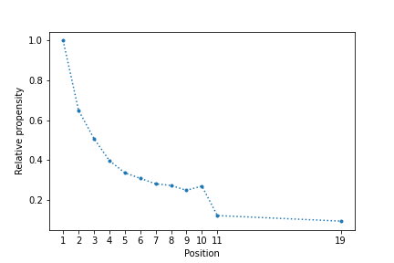
So, randomization is what we did at Thumbtack. Across half of our traffic, for each search we randomly picked a pair of adjacent professionals to swap. That little bit of variation helps us estimate the position bias between any two adjacent ranks, and by extension, the position bias between all ranks.
It was easy and it worked.
It gave us very clean and sensible estimates of position bias factors, it didn’t cost us anything except slightly subpar ranking (which is not even that subpar if we have some modesty about how accurately our ranker was able to order adjacent pairs), and we were able to follow it up with an IPS-based ranker that gave us significant improvements to business metrics. We were even able to use those derived position bias factors for other use cases outside of ranking.
If instead we had gone with a purely observational approach:
Even in the best case, it might not derive as accurate position bias factors as a randomized experiment would
There is a substantial chance that it fails badly, giving very inaccurate position bias estimates and a biased relevance model
If it fails badly, we wouldn’t necessarily know — not until trying it on customers
There are some caveats to the PBM. Like any model, it will give poor results to the extent that its assumptions are incorrect. In particular, the separability hypothesis and the lack of quality-of-context effects are key assumptions. Coming full circle on this post and the last one, IPS with randomized position bias factors won’t fix misspecification.
But there are other advantages, too. IPS has been around for a while, so there is plenty of public code out there that actually works. It has a good track record, with a behavior model that is just expressive enough to capture key dynamics. We also won’t need to second guess ourselves on whether our models worked or not, to the extent that we use randomized data to test our model fit. Simplicity in both the behavior and ML models, combined with unbiased randomized evidence, is very reassuring to everyone involved. This is a good practical choice.
[1] Dupret, G., & Piwowarski, B. (2008). A user browsing model to predict search engine click data from past observations. SIGIR '08.
[2] Joachims, T., Swaminathan, A., & Schnabel, T. (2017). Unbiased Learning-to-Rank with Biased Feedback. Proceedings of the Tenth ACM International Conference on Web Search and Data Mining.
[3] Joachims, T., Granka, L.A., Pan, B., Hembrooke, H., Radlinski, F., & Gay, G. (2007). Evaluating the accuracy of implicit feedback from clicks and query reformulations in Web search. ACM Trans. Inf. Syst., 25, 7.
[4] Wang, X., Golbandi, N., Bendersky, M., Metzler, D., & Najork, M. (2018). Position Bias Estimation for Unbiased Learning to Rank in Personal Search. Proceedings of the Eleventh ACM International Conference on Web Search and Data Mining.
[5] Aslanyan, G., & Porwal, U. (2019). Position Bias Estimation for Unbiased Learning-to-Rank in eCommerce Search. SPIRE.
[6] Schnabel, T., Swaminathan, A., Frazier, P., & Joachims, T. (2016). Unbiased Comparative Evaluation of Ranking Functions. Proceedings of the 2016 ACM International Conference on the Theory of Information Retrieval.
The PBM exists at least as far back as 2008, in Dupret & Piwowarki, but I haven’t done an exhaustive search to find out exactly how far back it goes.
See Schnabel et al. for a more thorough discussion of ranking metrics [6]
Note that the demo in my last post avoided this effect because the examples did not have correlation between features or correlation between the positive features and rank.
An underrated point, in my opinion. It’s one thing to hypothesize that a behavior model is true and position bias factors are intrinsic to customer behavior, it’s another to trust in the model absolutely even if we served entirely random rankings.