The position bias problem, with code
Explaining the ranking problem and showing pitfalls of estimating on observed data

Let’s talk about ranking. Ranking is something I have worked on, among other problems, nearly continuously for the last four years. I recently wrote up a small paper sharing a portion of that work, but before I get into any of that material I want to spend a bit of time thinking through why this is a challenging problem at all. This post comes with a notebook for demonstration.
Once you start working on ranking, you see ranking everywhere. Google Search is a ranked list of links. Amazon is a ranked list of products. And of course Thumbtack is a ranked list of professionals. Sometimes the product orders the list top-to-bottom, sometimes left-to-right, sometimes in a grid. Sometimes the list contains multiple types of items intermixed. The common thread is that we have many results to consider and the order in which we present them matters a lot.
Ranking bias
We don’t need infinite search results. We might not even need 100, or sometimes even 10. We have a limited willingness to scroll and evaluate. That’s actually why ranking matters in the first place. But it creates a big problem for model building, that ranking matters yet the actual rank of an item is not intrinsic and permanent. Instead we choose it. The most important factor affecting clicks is one that is in our control.1
The image below, taken from my paper, shows a typical conversion curve with rapidly diminishing conversion by position.
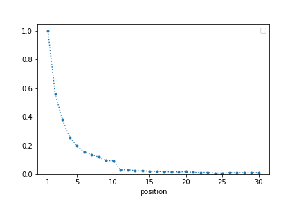
Conversion decreases by position. Part of that is by design, because we try to rank the best items at the top. Part of it is because users prefer the most immediate results and will not browse indefinitely. Disentangling those two effects can be very challenging.
Models that ignore position
Suppose we build a model that predicts click, using various features that do not include position, with each item from every search treated as an independent observation (or row) in the model.2 Since position does matter but is not directly modeled, models that find good proxies for position will have better fit. In an extreme case, imagine our search data comes from an algorithm that sorts purely on item titles, alphabetically, with no effort to sort on relevance to users. Title would have a strong correlation with clicks, because title causes rank and rank causes clicks. Our model could learn an approximation of alphabetical ranking.
This would be fine if we wanted to predict outcomes holding the ranking constant. If the ranking stays unchanged, the model can predict future clicks as well as it predicts historical clicks. But the exact thing we want to do is change the ranking. Suppose we switch to ranking by rating. User metrics may improve substantially (since rating is actually a useful criteria that users care about), yet our model would predict the opposite. It will predict degraded outcomes of the new ranker, because the new ranker will have less correlation with alphabetical titles, and the model has learned to prioritize titles. We want to de-bias the effect of position from the model, ideally discovering a true model of relevance.
I put together a demo of a similar scenario in the notebook. I introduce two features: num_reviews (a normally distributed integer) and avg_rating (on a 0-5 scale), and an outcome of interest, has_click. Users only care about rating and position. Unfortunately the ranker sorts by reviews, which is something users do not care about.
The image below shows some example data from the first randomly generated search. Despite variance in avg_rating, click probability is almost monotonically decreasing with position.

We can fit a model to this data using num_reviews and avg_rating as features. The model puts a lot of emphasis on num_reviews, even though it isn’t causal.3 The model has good in-sample fit, and would fit well on any similar data generated from the same ranker.
But what happens when we change the ranker? Let’s take the most challenging case: where we exactly reverse the ranking algorithm, now ranking ascending by number of reviews. The model performs horribly on this new data, even though customer behavior doesn’t change.
If there’s one chart that illustrates this most clearly, it is this one of predictions actually increasing as position worsens, while clicks drop substantially with position.
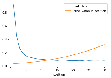
Our model did not generalize, because it took advantage of num_reviews as a proxy that was highly correlated correlated with has_click, but was not a truly causal feature.
Models with position as a feature
You might think that this problem has an obvious solution: use position as a feature. That’s what I thought too. It’s not a rare approach either [2]. But it has a checkered history.
One critique is that “the position feature cannot be used during inference time when a collection of documents must be scored to determine their positions in the presented ranking” [3]. This is a bit of an odd critique, since this structure allows us to test any counterfactual position — including, most notably, the 1st position.
Another critique, from Wang et al. at Google, is that “when there is a high correlation between [positions and regular ranking features], the attribution can be arbitrary” [5]. Yet this is the problem of multicollinearity in general. When features are collinear but not perfectly collinear, we can still tease apart their separate effects if we have enough data and an appropriate model specification.
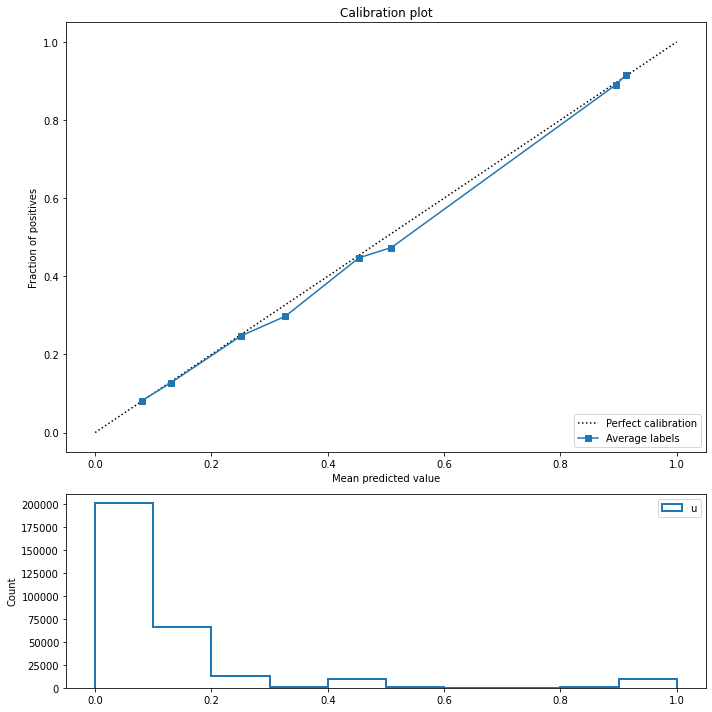
I show that next when I fit a logistic model that adds inverse_position as a feature. Since the behavior model follows a logistic specification, the logistic model is able to identify nearly the exact coefficients despite the correlation between position and num_reviews. Note that the absolute value of num_reviews is not important, but its relative value in the search is what determines position, so it is less useful for fit than inverse_position. The model learns that inverse_position matters, avg_rating matters somewhat, and num_reviews does not matter at all. It performs well even when we change the ranking function, with superb calibration and accurate predictions by position.

This shows that in some scenarios (caveat for next time: not all!) it is very possible to fit a ranking problem with a naive model.
Nevertheless, Wang et al. finds that the embedded model not only performs worse than their proposed method, but even does worse than a model without position. There is a reason why, and it isn’t because position is unavailable or that position is collinear with the features that determine ranking.
Misspecified models
In my demo a logistic model was well-suited for fitting a logistic behavior model. This was designed to demonstrate compatibility in trivial cases, but the real world is rarely so trivial. Next I created a very different behavior model, where click likelihood is defined by position bias multiplied by a logistic relevance probability.
A new logistic model did a poor job of finding the true model, since it fundamentally isn’t expressive enough to use a multiplicative relationship. It can fit the observed data to a decent extent, but it needs to use num_reviews to do so, leading to very poor performance under the alternative ranker.
If we then switch to a much more expressive model, a gradient boosted decision tree (GBDT), we see a substantial improvement. Yet the GBDT still performs poorly when tested on a new ranker with reversed ranking. Not as badly as the logistic model, but still poorly.
Accurate performance on the training sample does not imply generalization under other rankers. We likely need a more expressive model (maybe even just a GBDT that is less underfit) and ideally more training data, especially if building a real model that has more complex customer behavior and corresponding more features.
This provides one hypothesis why the embedded model in Wang et al. might have performed so poorly: They restricted its functional form to prevent interactions between position and other features, severely handicapping its expressiveness relative to their own method.
Ironically, specification problems might be exactly where their own approach struggled too.
A strong attempt at an observational position bias model
Wang et al. use a common functional form to model rankings, with a multiplicative position bias much like in the second part of my demo. They have search data from Gmail and Google Drive to test their models on, and they have data from a randomized experiment that they can treat like ground truth for position bias factors.4
They use an expectations-maximization (EM) approach to fitting the model, with a GBDT for the maximization step. Given a set of position biases, they run a GBDT to fit the data and identify relevance, then they update the position biases to reflect the relevance estimates from the GBDT, then fit the GBDT again, and so forth until the result converges and they minimize total loss. Although the EM method is different than the single iteration model with position factors that I described earlier, this is conceptually a similar approach: take observed data and fit it as closely as possible.
How well does it do? On Gmail data it looks great.

In the figure, “Empirical” is the raw decay in clicks by position, “Embedded” is the single iteration model, “EM” is their approach, and “RandPair” is approximately the right answer based on randomized experimentation. The Empirical curve is much steeper than the others, because clicks decay both due to position bias and because the ranker is successful at ordering the best items first. EM is a lot closer to RandPair than Embedded is, as evidence that EM out-performs the Embedded method.
This seems like a success story for the method. That it, until we look at Figure 2b.

The Google Drive data has a much sharper empirical curve, but much less true position bias. The EM model still does better than the embedded model, but not all that much better, and both are far from correct.
If a method is only successful on one of two datasets used in its own paper, you can bet that it won’t extrapolate well to other studies. The EM method did not work well for Aslanyan & Porwal, who explain “this method uses the ranking features to estimate relevances and can result in a biased estimate of propensities unless the relevance estimates are very reliable, which is difficult to achieve in practice” [5]. Likewise, some of the writers of Wang et al. are coauthors in Agarwal et al., in which the EM method performs poorly and they backtrack quickly on it. That paper eloquently explains that “defining an accurate relevance model is just as difficult as the learning-to-rank problem itself, and a misspecified relevance model can lead to biased propensity estimates” [6].
In other words, it comes down to specification. If we have the right functional form for behavior, including the causal features, we can fit position bias with observational data. If we have the specification a bit wrong, we might be wildly wrong with our position bias estimates and our model will fail when generating counterfactual estimates for other rankers. Finding the right model might be the tough part.
Conclusion
While many writers have tersely dismissed the possibility of fitting a model with position as a feature, I feel that the story is a little more complicated. This approach isn’t guaranteed to fail. I would not be surprised if much more expressive models sometimes do fine. The simple approach of using position in a model may be simultaneously overrated by people new to the problem while underrated in the literature.
Regardless, we have safer methods that incorporate random variation instead of purely observational data. I’ll get into those soon enough. If you don’t want to wait, go give my paper a read.
[1] Pearl, J. (1995). Causal diagrams for empirical research. Biometrika, 82, 669-688.
[2] Huyen, C. (2022). Chapter 8: Data Distribution Shifts and Monitoring. In Designing Machine Learning Systems (1st ed., pp. 233–236). O'Reilly.
[3] Agarwal, A., Wang, X., Li, C., Bendersky, M., & Najork, M. (2019). Addressing Trust Bias for Unbiased Learning-to-Rank. The World Wide Web Conference.
[4] Wang, X., Golbandi, N., Bendersky, M., Metzler, D., & Najork, M. (2018). Position Bias Estimation for Unbiased Learning to Rank in Personal Search. Proceedings of the Eleventh ACM International Conference on Web Search and Data Mining.
[5] Aslanyan, G., & Porwal, U. (2019). Position Bias Estimation for Unbiased Learning-to-Rank in eCommerce Search. SPIRE.
[6] Agarwal, A., Zaitsev, I., Wang, X., Li, C., Najork, M., & Joachims, T. (2019). Estimating Position Bias without Intrusive Interventions. Proceedings of the Twelfth ACM International Conference on Web Search and Data Mining.
The outcome is called a click in the literature, but in practice could be any positive outcome.
This is called a pointwise approach, as opposed to pairwise or listwise.
All this talk of causality might astutely remind you of the literature on causal graphical models, where are very much appropriate in this context. This is the problem of confounding bias in the influential works of Judea Pearl [1].
That randomized approach sounds handy, right? Foreshadowing…