Why we discard useful sample
Diminishing returns to sample, combined with computation and engineering cost, leads to practical limits on sample sizes.

In my last post I discussed the scenario where data accumulates over time and data drift gives us a preference for recency. Together these can result in small optimal sample sizes. Today I want to discuss how we can prefer to discard data even in static domains without drift, in the lucky case where we have substantial sample at our disposal.
Imagine a fairly static domain with no mechanism for behavioral change: object recognition in images. A cat is always a cat.1 More sample might seem strictly better than less sample. With more sample we can measure relationships more precisely and avoid the problem of “noisy” absolute rarity [1]. We can represent complex behavior with sufficiently parameterized models (e.g. deep neural networks with layers tailored for the problem space). We need enough observations to learn those parameters accurately enough and not have them subject to too much random variation.
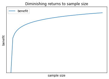
The effect of sample size on model performance is complicated. See Viering & Loog for a lovely, nuanced discussion [2]. Most typically, performance follows a power law relationship with sample size (“for most models, the power law offers the best fit”), with diminishing returns particularly after some boundary. Hestness et al. also supports this power law relationship, stating “our empirical results show power-law generalization error scaling across a breadth of factors” [3].
In chart form, it can look like this:
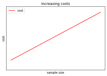
Meanwhile, training time complexity is often linear or worse than linear. You can see some complexity results consolidated here [4]. Plotting a linear cost:
You can see where this is going. Eventually cost will exceed benefit.
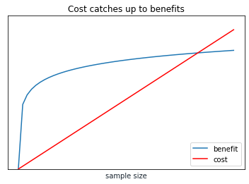
I made one sleight of hand with that last chart: The benefit line will naturally be in terms of model performance, while the cost line will be in terms of time complexity. I’m making an assumption that I can create comparable units from both. Let’s say that unit is revenue, and both benefits and costs have linear relationships with revenue.2 For example, improved model performance can lead to better outcomes in product applications, while time complexity can directly lead to compute costs and people costs. The exact point of intersection may vary, but the general trend remains.
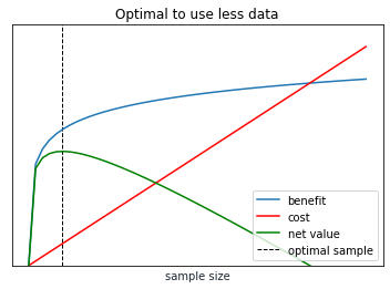
The appropriate amount of sample is then the point with the maximum positive difference between benefit and cost, like so:
Will parallelism save us?
Parallelism complicates this story, both at the small scale of vector computation and cache efficiency on processors and in the large scale of distributed computing in data centers. We might think that with parallel computing we have constant time complexity, in which case more sample is always better:
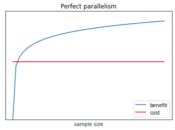
Hypothetically an ideal parallel system might have constant training time, basically the training time of any single node. However, to actually realize this ideal we need overhead that does not increase with the number of nodes. We also need similar ideal parallelism properties at every stage, including dataset generation, feature processing, and training. This is a challenging ideal to reach. Instead we might still see a linear relationship that is less steep than without parallelism.
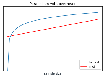
Kennedy et al. is an example of researchers testing a basic parallel system that finds linear performance with any node size, shown in their Figure 2 [5].
That system is not as polished as cutting edge distributed frameworks at companies like Google, and in particular if we have efficient autoscaling of nodes then our time complexity line flattens out more.
Regardless, sooner or later every system will hit some boundary where it cannot support further scaling. At that point we need to adapt the system or invent a new one. This creates an immense discontinuity in time with respect to sample size, as passing that boundary means not minutes of more training but more like months of development work.
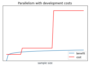
Collectively these boundaries may mean that even advanced distributed systems behave with linear (or worse) complexity in aggregate.
Putting it together
The value of more sample diminishes rapidly and may reach an asymptote, while training cost grows steadily.
Where this can lead to worse models is when the training time delays model evaluation, crowds out time that could be used for feature investments or architectural changes, or when the team has to focus on scaling a complicated training system rather than on designing effective models. And while model runs, modelers, and engineers can all be parallelized they all have their own scaling problems.
New technology pushes out the frontier of optimal sample, and the easiest choices are when those improvements come for free due to improvements in libraries or external platforms. Internally every company has limitations on how much technology investment is efficient to build in-house.3
At some point more sample is not worth the incremental effort.
The ideal amount of training data depends on the problem domain and is intricately tied to training infrastructure and team processes. For many teams the exact optimum is not worth ruminating on. Somewhere in the code you can usually find a magic number that specifies a fixed training size or duration.4 People in these teams may be apologetic about discarding sample and they might treat the practice like a guilty secret, but it is fairly easy to see how their behavior can be optimal within a framework that considers scaling costs.
Teams may test changing the magic number dramatically, doubling or (more rarely) halving it. Doing that occasionally to move towards a local optima for the problem domain might be a more efficient use of time than trying to precisely identify the ideal sample size, especially considering that ideal sample size could change with new features, new architectures, or concept drift. Simple approaches pay off.
[1] Weiss, G.M. (2004). Mining with rarity: a unifying framework. SIGKDD Explor., 6, 7-19.
[2] Viering, T.J., & Loog, M. (2021). The Shape of Learning Curves: a Review. ArXiv, abs/2103.10948.
[3] Hestness, J., Narang, S., Ardalani, N., Diamos, G.F., Jun, H., Kianinejad, H., Patwary, M.M., Yang, Y., & Zhou, Y. (2017). Deep Learning Scaling is Predictable, Empirically. ArXiv, abs/1712.00409.
[4] Computational complexity of machine learning algorithms. The Kernel Trip. (2018, April 16). https://www.thekerneltrip.com/machine/learning/computational-complexity-learning-algorithms
[5] Kennedy, R.K., Khoshgoftaar, T.M., Villanustre, F., & Humphrey, T. (2019). A parallel and distributed stochastic gradient descent implementation using commodity clusters. Journal of Big Data, 6, 1-23.
There is actually a little bit of drift here, as concepts change. Images of phones from 50 years ago might not be a great corpus for identifying modern telephones. Even with the example of cats, we have breed new cat breeds for a long time and we will keep doing so. But compared to something like spam, visual concepts are orders of magnitude more static
We can easily imagine a scenario where that isn’t the case, where model performance beyond a threshold does not add more value (in which case the curves may intersect even earlier) or we have logarithmic pricing for compute time (in which case the curves may or may not intersect at all)
This is true even at Google, yet Google is simultaneously an example of a company that regularly pushes out the frontier of its ML systems. Innovation dynamics at a company of that scale, and of the ecosystem as a whole, might make for a post on their own.
That magic number might be 14, or 30, or 365, which all have meaningful interpretations to humans as durations of days but don’t have any intrinsic benefits over, say, 13 or 31 or 366