
When more sample leads to worse models
When more sample leads to worse models
The importance of recency might mean that more historical sample hurts out-of-time model performance

In my last post I discussed sample balancing. A recurring theme and underlying motivation for balancing is having too little sample. In many predictive problems, especially small sample ones, we crave more data. More sample can give us more signal for prediction.
However, more sample isn’t always better, both in small sample and large sample problems. In this post I want to cover one particular scenario: where data recency matters and when we can’t control the incoming volume of sample.
In some domains the practical way to accumulate data is through time. Using spam prediction as an example, we get more data as time goes by and users send and receive emails.1 This differs from domains such as image recognition, where we can pay for quality labeled images. How much of history should we use for our samples? One answer could be “all of it”, as far back in history as we have data or as much data as we can process.
We also can have drift, where human behavior changes, we have a different composition of users, or when our product behaves differently. The data is not stationary. In many domains our most recent data is the most representative of the near future, and a combination of using recent data plus regularly updating models leads to strong ongoing performance.
Due to drift we often want to use the most recent data, and due to the user-generated nature of data we add more data only through the passage of time. Additional data may give us more information to identify predictive relationships, but may also have higher drift relative to the near future. We might have to trade-off between these two contrasting effects. Or maybe not: maybe historical sample adds diversity and helps the model generalize.
How do we know the ideal sample size? We can get some insight through simulations, evaluating historical counterfactuals from different periods with varying sample windows.
One could start with a corpus in which we try different durations of training windows. We would split train and test on a date to mimic the scenario of fitting a model on prior data and then using the model on the near future. Then we could choose whichever duration of sample size gives the best performance on the (fixed in time) future test sample.
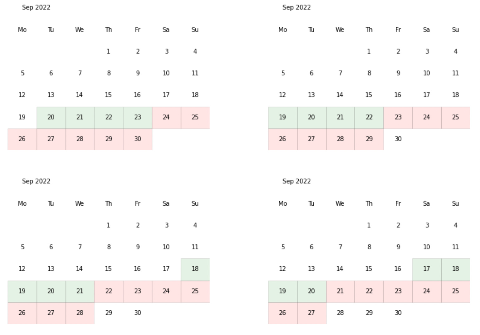
For example, say we perform this exercise on October 1st, 2022, with complete data on dates through September 30. If we choose a 7 day evaluation sample we would use the last 7 days (September 24th through 30th) as a test sample, and we would try different lengths of training sample. For one day we would use September 23rd, for two days September 23rd and 22nd, and so forth. The first four are shown below:2

The problem with this approach is that it has high variance because it uses a fixed test window and one set of days per duration. The winning duration could prevail for any number of reasons that do not generalize to other periods or future iterations of the model.
Instead we can use that technique, but applied to every feasible start date. This vastly reduces (but doesn’t entirely eliminate) the risk of poor generalization.
To evaluate the effectiveness of 4 days of sample, for example, I create a sample and model from every possible 4 day window. Then I test out-of-time relative to those times, in the near future after each model. If I have 100 days of historical data, and I choose to look at a 7 day future test sample, I can generate 100 - 7 - 4 = 89 samples of 4 days of training data each. Again using my example of data through September 2022, the first four periods are shown below.
Each sample has an associated loss value on its respective test period. I can average or look at the distribution of those 89 losses. Next, I can follow a similar process for 5 days, 6 days, and any other length.3
In Pythonic pseudocode, it looks like this:
for duration in durations:
  duration_losses = []
  for start_date in possible_start_dates(duration):
    model = construct_model(duration, start_date)
    loss = calculate_test_loss(model, duration, start_date)
    duration_losses.append(loss)
  average_loss = mean(duration_losses)
  report_average_loss_for_duration(duration, average_loss)
The chart below shows actual results for one of my models. I showed it here with two specifications, at the time demonstrating how feature selection has caveats too. But that’s a topic for another day. Let’s just focus on how both blue and green lines have a similar trend.
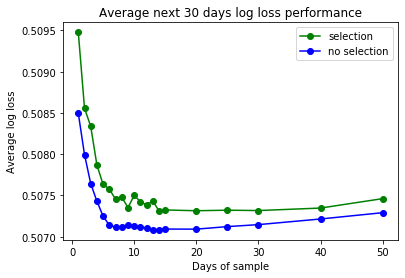
Performance improves rapidly for the first few days of incremental data, then after about a week of data further improvements are very marginal and shortly afterwards start to reverse.
Of course this is not the only way to incorporate recency preferences. We can weigh our data in batch model building or online updating. Which would still leave us with the problem of identifying the appropriate recency weights. We can fit an exponential decay rate, with a single decay parameter to find. We can tune that decay parameter using a similar method to the above.
Many find it simpler to use a fixed sample duration. Even with many caveats to this simulation approach, it gives some insight on how our problem space depends on sample size and whether we have drift and should prioritize recency.
Stay tuned for my next post, where I talk through scenarios where sample size can be damaging even without drift.
For example, at Google we could try to convince people to send more emails so we have more spam data, yet this would be challenging and total email volume would have been hard or costly for us to control.
You may want to be careful to align the different time windows. We are able to create 70 periods of single-day samples, compared to only 50 periods of 20-day samples. This means that some of our evaluation windows for single-day samples happen earlier than the earliest evaluation windows for a 20-day sample (with some partial overlap). That might make for an unfair comparison if particular periods are easier or harder to predict from their recently preceding data.