
Entropic emanations

We all love log loss. For problems with binary labels it makes such intuitive sense. Loss is 0 when we predict the true outcome with 100% certainty and loss is infinite when predicting a 0% likelihood (which means that our model has been unequivocally proven wrong). Log loss is differentiable and simple to backpropagate. It is a proper scoring function, meaning that it incentivizes honest prediction instead of incentivizing any intentional inaccuracies.1 Log loss is symmetric, such that if we incorrectly predict 80% positive likelihood on a negative observation our penalty is the same as predicting 20% positive likelihood for a positive observation. As we’ll cover below, log loss is firmly grounded in probability theory and has intrinsic meaning. What’s not to like?
We can generalize log loss to multiclass problems, where there are more than two possible outcomes that are mutually exclusive and collectively exhaustive. Probabilities across the classes should sum to 1, even if it means one of the classes has to be “other”. Consider a horse race with 10 horses. One must win the race, and ahead of the race we could generate probabilities of each winning. In this multiclass setup we use cross entropy for our loss, which means that again we look at how far off we are from the outcome, on a log scale, such that cross entropy is likewise bound by 0 and infinity.
For n observations with m different classes, with binary outcome y and predictions P(y), mean cross entropy loss is:
Log loss is just cross entropy when restricted to only two classes. If we define negatives as class 0 and positives as class 1, then cross entropy simplifies to log loss:
Did you notice that cross entropy ignores the negative classes?
There is one thing that bothers me about cross entropy. Holding the probability of the true class fixed, it doesn’t matter how probability is distributed among the remaining classes. Consider again a horse race of 10 horses where horse #1 won the race. Classifier A predicted 10% likelihood for each of the 10 horses, while classifier B predicted 10% for horse #1, 90% for horse #2, and 0% for the remaining eight horses. This is shown below.2
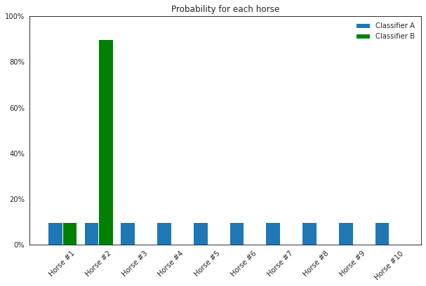
Both classifiers have the same cross entropy loss, -log(0.1). Cross entropy only counts the prediction for horse #1.
An alternative way of writing log loss in binary problems is to take the class that didn’t happen, consider its positive probability as x, and penalize by -log(1 - x). That’s correct. Yet if we tried to generalize that to multiple classes by calculating for each negative class and summing the loss, that would be incorrect. Instead we need to add all the probabilities of negative classes together first and use that as x in the equation. The individual probabilities for negative classes do not matter.
This doesn’t sit well with me.
The intuition I built up was that log loss cares about how wrong we are about all of our probability claims.
It feels unintuitive for part of our predictions to just not matter. I didn’t hand-pick examples that gave the same loss. Rather, any combination of probabilities that leave horse #1 with a 10% prediction all have the exact same loss.
Expecting a particular outcome 90% of the time and not seeing it feels more incorrect than expecting 10% from each of nine possible outcomes.
Cross entropy and likelihood
Cross entropy is derived directly from likelihood. Maximum Likelihood Estimation (MLE) can be a scary acronym and its equations can be a bit confusing. At its core, it just means that we should pick probabilities such that the outcomes we saw are as likely (according to our own chosen probabilities) as possible. In my horse racing example, given either set of probabilities I used as examples, the likelihood of what we observed (horse #1 winning) is 10%. If instead I predicted 20% for that horse, then the likelihood of the outcome was 20%, which is higher and better. The best I could have done is predict 100% chances for horse #1. MLE is the process of picking the maximum possible probabilities for the true outcomes.
When put that way, you might ask why we don’t always predict 100% for the outcomes that happened. We need a way to generalize to new circumstances. Continuing with our horse racing example, we need a model that can tell us win probabilities for different groups of horses, or even the same horses but across more races. If we build our model we will have a corpus of many races, and we typically will find that it is hard to ever be 100% certain. Additionally, we usually fit a small number of parameters to model our behavior, and it may be impossible to fit all data points with those parameters.3 Between these reasons, we end up with a likelihood value that is less than 100%.
From likelihood, we can take its log (“log likelihood”), which is a monotonic transformation such that maximizing log likelihood is a way to maximize likelihood. We can then negate the outcome, giving us negative log likelihood (which we just call “log loss” in the binary case or “cross entropy” more generally), which we can minimize. Minimizing log loss is the same as maximizing log likelihood.
Sidebar: Why just log, anyways?
We use log to make our gradient calculations easier.4 Multiplicative terms become additive on a log scale. However, even though solutions to maximization problems are invariant to monotonic transformations, the change could have ramifications on our learning. A lot of work goes into designing optimizers. Maybe we shouldn’t actually penalize on this specific log scale. Consider the example of focal loss for a case where different monotonic transformations do indeed lead to different results [2]. Or consider the success people have found using Mean Squared Error (MSE) in classification instead of cross entropy [3]. Really, we should use whatever works—but I’ll caveat that “whatever works” has now been heavily tailored to cross entropy loss.
The derivation of cross entropy all makes sense. So my qualm isn’t specifically with cross entropy, but rather with likelihood.
Likelihood is only about the probabilities of the events that occurred. It has nothing to say about the probabilities of outcomes that didn’t occur.5 And why would it? How can we have any framework to distribute the incorrectness between the negative classes? For any given observation, we don’t know which negative class is “more wrong” than another.
What could we change?
Let’s think about modifying cross entropy to care about negative classes.
I can think of at least two reasonable ways to do it:
Prefer equal probabilities among the negatives
Prefer negative probabilities to match event rates for each class
The first one is a uniform prior, while the latter is an event rate prior.
It’s normal for people to design loss functions with secondary objectives, sometimes in Bayesian terms. Regularization in loss functions is common. But that adds a preference for parsimony on the model parameters themselves, not on predictions from the model. I struggled to find any academic discussion of similar concepts, although I did find a nice StackExchange thread.
I’m not even sure if my approach makes sense. But that shouldn’t stop us; many ideas that didn’t have a logical design to them have succeeded in ML and only retroactively gained explanations.
Downsides
One of the intentional advantages of cross entropy is how simple gradient calculation is, and I’ll throw that out the window. I’m unsure of the actual ramifications on model fitting.
How much weight would I like to give to these priors? Not very much. If we have a large number of classes then our model’s loss might be dominated by the negative classes, limiting our ability to lower loss on the actual positive classes.
We actually start to see problems like this when we have multi-label classification, in which there can be more (or less) than one positive label per observation. For such models we use log loss for each possible label independently. There is a downside that “this positive-negative imbalance dominates the optimization process, and can lead to under-emphasizing gradients from positive labels during training, resulting in poor accuracy” [4].
Furthermore, varying probabilities for negative classes can actually be a good thing. Consider the classic MNIST dataset of handwritten digits. Ben Levinson has some examples of awful writing leading to borderline cases, including a 9 that looks like a 4, a 3 that isn’t far from a 2, 2s that might as well be 1s, etc. [5]. Probabilities can still be useful in this case, for understanding which other digits a handwritten digit is most similar to.
Handwritten digits are meant to have an absolute truth to them, such that there is no randomness about which number a person attempted to write. We can also consider outcomes where the true underlying process is probabilistic. My horse racing example is such a case, where there is real randomness in each horse race. There is an element of irreducible error. While I wanted to penalize a model more if a horse lost a race despite being given 90% chance of winning, it’s possible that the 90% probability was correct and we had an upset in the race due to random chance. And it’s unlikely that we have only one observation with that horse. Perhaps there were many other races in our dataset in which that horse won, and the model is calibrated.
Experiments
I’m far away from understanding this area at a deep level, but nothing stopped me from getting hands-on and playing around with some options. You can see my work in this notebook, where I define a few versions of loss functions that penalize on prediction discordance among negative classes.
I use the CIFAR-10 dataset, which has 60,000 images that each have one of 10 classes [6]. The classes are airplane, automobile, bird, cat, deer, dog, frog, horse, ship, and truck. I picked this dataset because it is small, well-known, the right answer is absolute, and the classes are fairly distinct from each other. This fits the use case of my loss functions. The labels are balanced, which also makes the choice of prior easy: I want uniform predictions across negative classes. I built intentionally simple models, purely for the convenience of speed, and I additionally save time by underfitting with few epochs.
I tried three loss functions. For all of them I start with a cross entropy loss on the correct class, and then calculate the ideal prediction for the negative classes. In one version I penalize by the log distance from target, much like log loss on the positive class. In another version I use absolute deviation, and in another absolute deviation times 10.
What happens? My custom loss functions have poor accuracy. The loss functions do lead to more consistency among the negative class labels, at the cost of lower predictions for the correct classes and worse overall accuracy. That’s not much of a surprise.
Maybe I need to fit the models a lot longer to compensate for the more complicated gradient surface of my loss functions. More generally, I wonder if my loss functions would only be useful on overspecified models.6 Essentially I want my compound loss to be lexicographic, in the sense that I would not trade off prediction on true classes at all for any improvement in balance among negative predictions. I’d like to first optimize probabilities on the correct classes as far as possible, and then balance probabilities on the negative classes as much as I can without sacrificing accuracy.
I’d like to repeat this exercise some day, but with far more epochs and more expressive models. Early results aren’t particularly convincing, but I’m not sure the idea is dead yet. If nothing else, I had some fun giving it a whirl.
[1] Gneiting, T., & Raftery, A.E. (2007). Strictly Proper Scoring Rules, Prediction, and Estimation. Journal of the American Statistical Association, 102, 359 - 378.
[2] Lin, T., Goyal, P., Girshick, R.B., He, K., & Dollár, P. (2017). Focal Loss for Dense Object Detection. 2017 IEEE International Conference on Computer Vision (ICCV), 2999-3007.
[3] Hui, L., & Belkin, M. (2020). Evaluation of Neural Architectures Trained with Square Loss vs Cross-Entropy in Classification Tasks. ArXiv, abs/2006.07322.
[4] Baruch, E.B., Ridnik, T., Zamir, N., Noy, A., Friedman, I., Protter, M., & Zelnik-Manor, L. (2020). Asymmetric Loss For Multi-Label Classification. 2021 IEEE/CVF International Conference on Computer Vision (ICCV), 82-91.
[5] Levinson, B. (2017, December 20). Comparing classifiers on the MNIST Data Set. Retrieved March 12, 2023, from https://benlevinson.com/projects/comparing-knn-svm-mnist
[6] Krizhevsky, A. The CIFAR-10 dataset. Retrieved March 12, 2023, from https://www.cs.toronto.edu/~kriz/cifar.html
[7] Vitay, J. Multi-class classification. Retrieved March 12, 2023, from https://julien-vitay.net/lecturenotes-neurocomputing/2-linear/5-Multiclassification.html
This sounds like an obvious property of loss functions, that we should never have an incentive to report a probability different than what we actually believe is the best estimate. But it’s not always the case! For a trivial example, mean absolute error (MAE) isn’t a proper scoring function [1]
The name for a distribution of probabilities is the Probability Density Function (PDF). In cases like this with discrete probabilities, it is a Probability Mass Function (PMF).
While fitting a model with fewer parameters than observations is a traditional practice, the alternative of intentionally overfitting models is becoming more popular. It even has its own Wikipedia page now!
See this nice derivation by Julien Vitay [7].
Except in the sense that cumulatively as they add up to 1 minus the probability of what did occur.
Coming full circle to an earlier footnote.